
An Introduction do Neural Networks: Solving the XOR problem
When I started AI, I remember one of the first examples I watched working was MNIST(or CIFAR10, I don’t remember very well). Looking for online tutorials, this example appears over and over, so I suppose it is a common practice to start DL courses with such idea. Although a very exciting starting point (come on, we are literally seeing a classifer recognizing images!), it kind of masks the math behind it and makes it harder to understand what is going under the hood (if you are a beginner). That is why I would like to “start” with a different example.
This example may actually look too simple to us all because we already know how to tackle it, but in reality it stunned very good mathematitians and AI theorists some time ago.
The 2-Variable XOR Problem
What is the XOR logical gate? Imagine two inputs that can assume only binary values each (0 or 1). The output goes to 1 only when both inputs are different. That is:
| x1 | x2 | y |
|---|---|---|
| 0 | 0 | 0 |
| 0 | 1 | 1 |
| 1 | 0 | 1 |
| 1 | 1 | 0 |
Now we must propose an artificial neural network that can overfit the dataset. That is, we should design a network that takes x1 and x2 as inputs and successfully outputs y.
Following the development proposed by Ian Goodfellow et al, let’s use the mean squared error function (just like a regression problem) for the sake of simplicity.
We already know what we should do. Now we should choose the model f(\(x\);\(\theta\)).
Theoretical Modelling (Let’s think for a while…)
Only one Neuron (A Linear Model)
Our first attempt will consider a linear model. Such model implements the following equation:
\(ŷ = f(\vec{x};\vec{w},b) = \vec{x}^{T}\vec{w}+b\).
Seems nice, isn’t it? Will it work? Well… unfortunatelly, no.
How can I now it beforehand? Let’s take a closer look to the expression. It is implementing a linear relation. Imagine f is a surface over the \(\vec{x}\) plane, and its height equals the output. The surface must have height equalling 1 over the points \([0, 1]\) and \([1, 0]\) and 0 height (it would be touching the plane) at points \([0, 0]\) and \([1, 1]\). Could a hyperplane behave this way? No, it cannot.
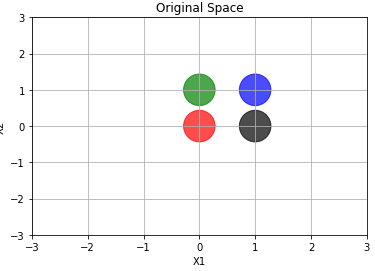
Another way of think about it is to imagine the network trying to separate the points. The points labeled with 1 must remain together in one side of line. The other ones (labelled with 0) stay on the other side of the line.
Take a look at the following image. I plotted each point with a different color. Notice the artificial neural net has to output ‘1’ to the green and black point, and ‘0’ to the remaining ones. In other words, it need to separate the green and black points from the purple and red points. It cannot do such a task. The net will ultimately fail.
More than only one neuron (network)
Let’s add a linear hidden layer with only two neurons.
\[ŷ = f^{(2)}(f^{(1)}(\vec{x}))\]or
\(ŷ = f^{(2)}(\vec{h};\vec{w},b)\) , such that \(\vec{h} = f^{(1)}(\vec{x};W,\vec{c})\).
Sounds like we are making real improvements here, but a linear function of a linear function makes the whole thing still linear.
We are going nowhere!
Notice what we are doing here: we are stacking linear layers. What does a linear layer do? How can we visualize its effect mathematically?
Before I explain the layer, let’s simplify a little bit by ignoring the bias term in each neuron (\(\vec{c}\) and \(b\)), alright?
Ok, now consider the following image (which can be found here):
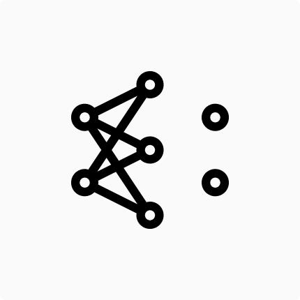
It is not our own net. Remember: We stacked layers with 2 neurons only, and here we have a hidden layer with 3 neurons. Even though it is not our neural network, it’ll be useful to mathematically visualize what’s going on.
Let’s focus only on the input and hidden layers. We can be sure this network was designed to a 2D input (like our example data), because there is two neurons in the input layer. Let’s call our inputs neurons using the following subscripts: \(i_{1}\) and \(i_{2}\). That means the first and the second input neurons. Watch out! When I say “the first” I mean “the higher”, “the second” then means “the lower”, ok?
The architecture consideration of the hidden layer chose three neurons. That is ok. There is not too much to talk about this choose. I will call the output of the three hidden neurons: \(h_1\),\(h_2\) and \(h_3\). And again, \(h_1\) is the output of the highest hidden layer neuron, \(h_2\) is the output of the hidden layer neuron in the middle and \(h_3\) is the output of the last hidden layer neuron.
I am repeating myself several times about the neurons’ positions because I want to be clear about which neuron I’m talking about.
Now let’s see the output of the first hidden layer neuron, that is, let’s see \(h_1\). We now \(h_1\) is a weighted sum of the inputs, which are written as \(\vec{x}\) in the original formulation, but we’ll use \(i\) so we can relate to input. In one equation:
\(h_1 = w_{1,1} * i_1 + w_{1,2} * i_2\).
don’t you forget we’re ignoring the bias!
In this representation, the first subscript of the weight means “what hidden layer neuron output I’m related to?”, then “1” means “the output of the first neuron”. The second subscript of the weight means “what input will multiply this weight?”. Then “1” means “this weight is going to multiply the first input” and “2” means “this weight is going to multiply the second input”.
The same reasoning can be applied to the following hidden layer neurons, what leads to:
\[h_2 = w_{2,1} * i_1 + w_{2,2} * i_2\]and
\(h_3 = w_{3,1} * i_1 + w_{3,2} * i_2\).
Now we should pay attention to the fact we have 3 linear equations. If you have ever enrolled in a Linear Algebra class, you know we can arrange these equations in a grid-like structure. If you guessed “a matrix equation”, you’re right!
The matrix structure looks like this:
\[\begin{bmatrix} h_1 \\ h_2 \\ h_3 \\ \end{bmatrix} = \begin{bmatrix} w_{1,1} & w_{1,2} \\ w_{2,1} & w_{2,2} \\ w_{3,1} & w_{2,3} \\ \end{bmatrix} \begin{bmatrix} i_1 \\ i_2 \\ \end{bmatrix}\]To simplify even further, let’s shorten our equation by representing the hidden layer output vector by \(\vec{h}\), the input vector by \(\vec{i}\) and the weight matrix by \(W\):
\(\vec{h} = W \vec{i}\).
If we connect the output neuron to the hidden layer, we have:
\(\vec{o} = M \vec{h}\), where \(\vec{o}\) is a 2D vector (each position contains the output of the output neurons) and \(M\) is the matrix that maps the hidden layer representation to the output values (the \(\vec{w}\) in the original formulation). Here, \(ŷ = \vec{o}\). Expanding it we have:
\(\vec{o} = M W \vec{i}\),
where \(MW\) gives another matrix, because this is just a matrix multiplication. Let’s call it A. Then:
\[\vec{o} = A \vec{i}\]Now suppose a different neural network, like the following (you can find it here):
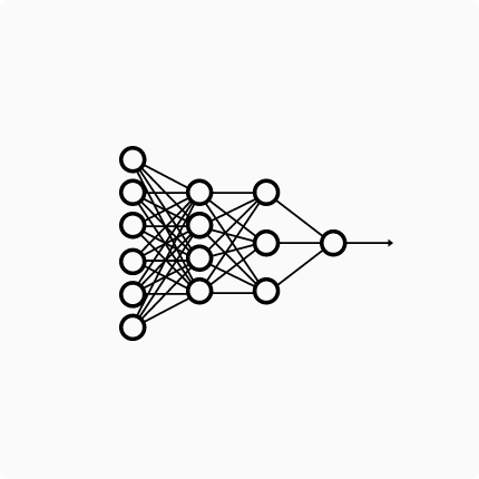
This network has only one output neuron and two hidden layers (the first one with 4 neurons and the second one with three neurons). The input is a 6-D vector. Again we are ignoring bias terms. Let’s see the shortened matrix equation of this net:
\(o = M H_1 H_2 \vec{i}\).
Here , the output o is a scalar (we have only one output neuron), and two hidden layers (\(H_2\) is the matrix of weights that maps the input to the hidden layer with 4 neurons and \(H_1\) maps the 4 neurons output to the 3 hidden layer neurons outputs). M maps the internal representation to the output scalar.
Notice \(M H_1 H_2\) is a matrix multiplication that results in a matrix again. Let’s call it B. Then:
\(o = B \vec{i}\).
Can you see where we’re going? It doesn’t matter how many linear layers we stack, they’ll always be matrix in the end. To our Machine Learning perspective, it means it doesn’t mean how many layers we stack, we’ll never learn a non linear behaviour in the data, because the model can only learn linear relations (the model itself is a linear function anyway).
I hope I convinced you that stacking linear layers will get us nowhere, but trust me: all is not lost. We just need another mechanism to learn non-linear relationships in the data. This “mechanism” I’ll introduce is called Activation Functions.
If you want to read another explanation on why a stack of linear layers is still linear, please access this Google’s Machine Learning Crash Course page.
Activation Functions!
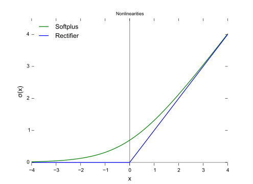
“Activation Function” is a function that generates an output to the neuron, based on its inputs. The name comes from the neuroscience heirloom. Although there are several activation functions, I’ll focus on only one to explain what they do. Let’s meet the ReLU (Rectified Linear Unit) activation function.
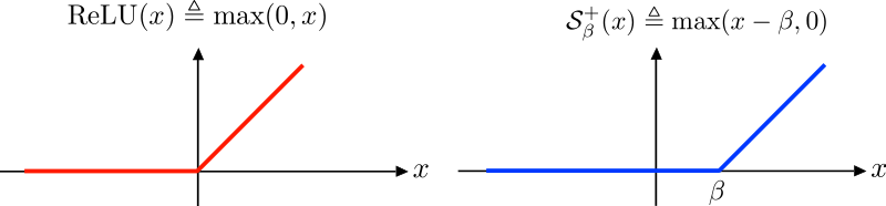
In the figure above we have, on the left (red function), the ReLU. As can be seen in the image, it is defined by the max operation between the input and ‘0’. It means the ReLU looks to the input and thinks: is it greater than ‘0’? If yes, the output is the input itself. If it is not, the output is zero. That said, we see every input point greater than ‘0’ has an height equaling its distance to the origin of the graph. That’s why the positive graph’s half is a perfect diagonal straight line. When we look to the other half, all x’s are negative, so all the outputs are zero. That’s why we have a perfect horizontal line.
Now imagine that we have a lot of points distributed along a line: some of them lie on the negative side of the line, and some of them lie on the positive side. Suppose I apply the ReLU function on them. What happens to the distribution? The points on the positive side remains in the same place, they don’t move because their position is greater than 0. On the other hand, the points from the negative side will crowd on the origin.
Another nice property of the ReLU is its slope (or derivative, or even tangent). If you have a little background on Machine/Deep Learning, you know this concept is fundamental for the neural nets algorithms. On the graph’s left side we have an horizontal line: it has no slope, so the derivative is 0. On the other side we’ve got a perfect diagonal line: the slope is 1 (tangent of 45º).
Here we have sort of a problem… what’s the slope at x=0? Is it 0 (like on the left side) or 1 (right side slope)? That’s called a non-differentiable point. Due to this limitation, people developed the softplus function, which is defined as \(\ln(1+e^{x})\). The softplus function can be seen below:
Empirically, it is better to use the ReLU instead of the softplus. Furthermore, the dead ReLU is a more important problem than the non-differentiability at the origin. Then, at the end, the pros (simple evaluation and simple slope) outweight the cons (dead neuron and non-differentiability at the origin).
Ok… so far we’ve discussed the 1D effect of ReLU. What happens when we apply ReLU to a set of 2D points?
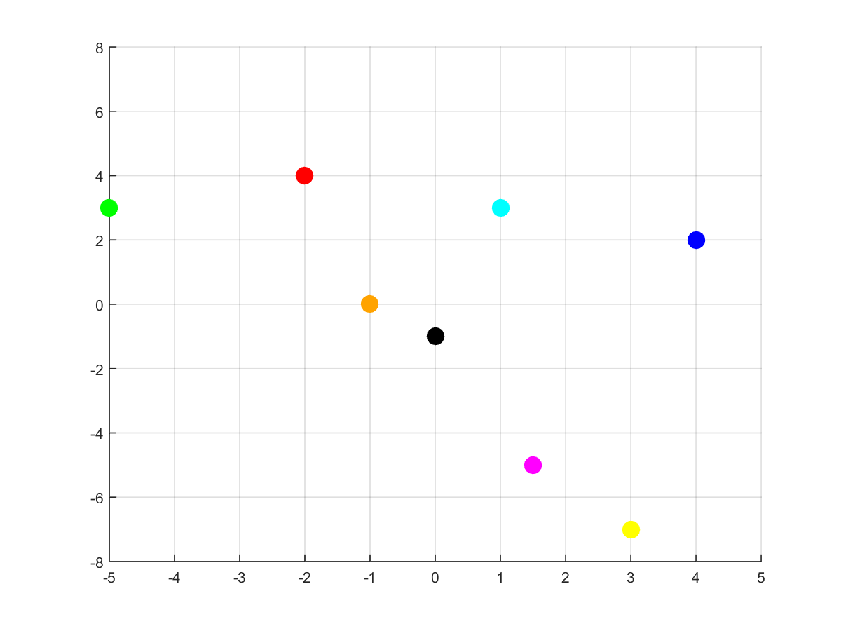
First, consider this set of 8 colorful points. Pay attention to their x, y positions: the blue ones have positive coordinates both; the green, red and orange ones have negative x coordinates; the remaining ones have positive x coordinates, but negative y ones. Suppose we applied ReLU to the points (to each coordinate). What happens?
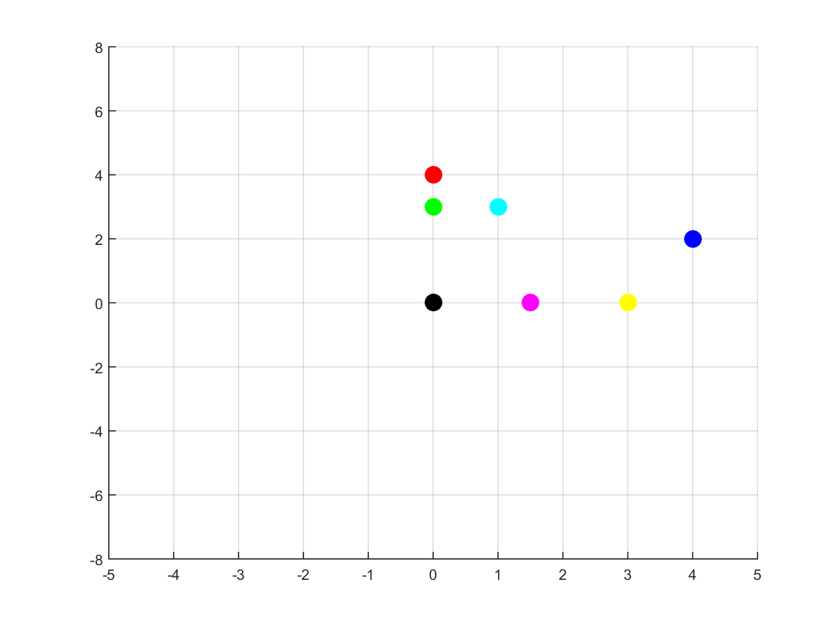
As we can see, the blue points didn’t move. Why? Because their coordinates are positive, so the ReLU does not change their values. The pink and yellow points were moved upwards. It happened because their negative coordinates were the y ones. The red and green points were moved rightwards. It happened due to the fact their x coordinates were negative. What about the orange point? Did it disappear? Well… no. Note every moved coordinate became zero (ReLU effect, right?) and the orange’s non negative coordinate was zero (just like the black’s one). The black and orange points ended up in the same place (the origin), and the image just shows the black dot.
The most important thing to remember from this example is the points didn’t move the same way (some of them did not move at all). That effect is what we call “non linear” and that’s very important to neural networks. Some paragraphs above I explained why applying linear functions several times would get us nowhere. Visually what’s happening is the matrix multiplications are moving everybody sorta the same way (you can find more about it here).
Now we have a powerful tool to help our network with the XOR problem (and with virtually every problem): nonlinearities help us to bend and distort space! The neural network that uses it can move examples more freely so it can learn better relationships in the data!
You can read more about “space-bender” neural networks in Colah’s amazing blog post

More than only one neuron , the return (let’s use a non-linearity)
Ok, we know we cannot stack linear functions. It will lead us anywhere. The solution? ReLU activation function. But maybe something is still confusing: where it goes?
I believe the following image will help. This is the artificial neuron “classic” model (classic here means we always see it when we start doing Machine/Deep Learning):

Recall our previous formulation: \(ŷ = f^{(2)}(\vec{h};\vec{w},b)\) , such that \(\vec{h} = f^{(1)}(\vec{x};W,\vec{c})\).
Here, a “neuron” can be seen as the process which produces a particular output \(h_i\) or \(ŷ_i\). Let’s focus on the \(h_i\). Previously it was explained that, in our context, it equals :
\(h_i = w_{i,1} * i_1 + w_{i,2} * i_2\).
Here, \(w_{i,j}\) are the weights that produces the i-th hidden-layer output. The i elements are the inputs (the x in the image). The transfer function comprises the two products and the sum. Actually, it can be written as \(h_i = \vec{w_i} \vec{i}\) either, which means the inner product between the i-th weights and the input (here is clearer the transfer function is the inner product itself). The input \(net_j\) is \(h_i\), and we’ll finally deal with the activation function!
In the original formulation, there’s no non-linear activation function. Notice I wrote: \(\vec{o} = ŷ = M * \vec{h}\) .
The transformation is linear, right? What we are going to do now is to add the ReLU, such that: \(\vec{o} = ŷ = M * ReLU( \vec{h} )\). Here, the threshold \(\theta_j\) does not exist.
So far it was said the activation function occurs after each inner product. If we think the layer as outputing a vector, the activation funcion is applied point-wise.
Visualizing Results (Function Composition)
The model we chose to use has a hidden layer followed by ReLU nonlinearity. It implements the global function (considering the bias):
\(f(\vec{x};W,\vec{c},\vec{w},b) = \vec{w}^{T} max\{0,W^{T}\vec{x}+\vec{c}\}+b\) .
A specified solution to the XOR problem has the following parameters:
W= \(\begin{bmatrix} 1 & 1 \\ 1 & 1 \\ \end{bmatrix}\),
\(\vec{c} = \begin{bmatrix} 0 \\ -1 \\ \end{bmatrix}\),
\(\vec{w} = \begin{bmatrix} 1 \\ -2 \\ \end{bmatrix}\),
and b = 0.
Let’s visualize what’s going on step-by-step.
First Transformation for Representation Space
What means Representation Space in the Deep Learning context? We can think the hidden layer as providing features describing \(\vec{x}\), or as providing a new representation for \(\vec{x}\).
When we apply the transformation \(W^{T}\vec{x}\) to all four inputs, we have the following result
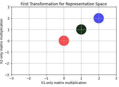
Notice this representation space (or, at least, this step towards it) makes some points’ positions look different. While the red-ish one remained at the same place, the blue ended up at \([2,2]\). But the most important thing to notice is that the green and the black points (those labelled with ‘1’) colapsed into only one (whose position is \([1,1]\)).
Second Transformation for Representation Space
Now let’s add vector \(\vec{c}\). What do we obtain?
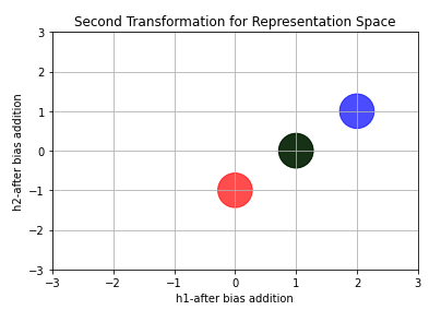
Again, the position of points changed! All points moved downward 1 unit (due to the -1 in \(\vec{c}\)).
Final Representation Space
We now apply the nonlinearity ReLU. It will gives us “the real” Representation Space. I mean… the Representationa Space itself is this one. All the previous images just shows the modifications occuring due to each mathematical operation (Matrix Multiplication followed by Vector Sum).
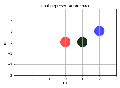
Now we can draw a line to separate the points!
Last Linear Transformation in Representational Space
The last layer ‘draws’ the line over representation-space points.
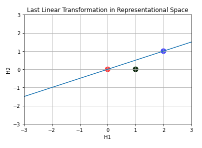
This line means “here label equals 0”. As we move downwards the line, the classification (a real number) increases. When we stops at the collapsed points, we have classification equalling 1.
Visualizing Results (Iterative Training)
We saw how to get the correct classification using function composition. Although useful for visualizing, Deep Learning practice is all about backprop and gradient descent, right?
Let’s see what happens when we use such learning algorithms. The images below show the evolution of the parameters values over training epochs.
Parameters Evolution
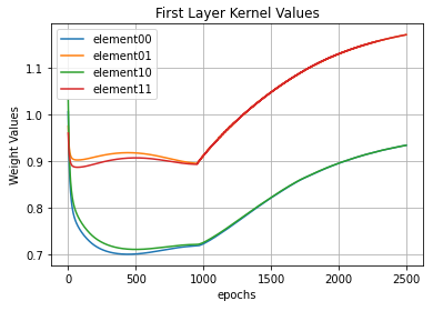
In the image above we see the evolution of the elements of \(W\). Notice also how the first layer kernel values changes, but at the end they go back to approximately one. I believe they do so because the gradient descent is going around a hill (a n-dimensional hill, actually), over the loss function.
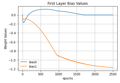
The first layer bias values (aka \(\vec{c}\)) behave like the first layer kernel kinda.
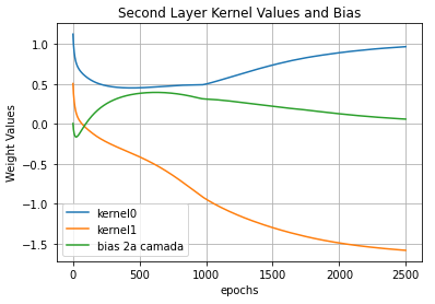
The main lesson to be understood from the three images above is: the parameters show a trend. I mean… they sorta goes to a stable value. Paying close attention we see they’re going to stabilize near the hand-defined values I showed during the Visualizing topic.
“The solution we described to the XOR problem is at a global minimum of the loss function, so gradient descent could converge to this point.” - Goodfellow et al.
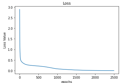
Below we see the evolution of the loss function. It abruptely falls towards a small value and over epochs it slowly decreases.
Representation Space Evolution
Finally we can see how the transformed space evolves over epochs: how the line described by \(\vec{w}\) turns around trying to separate the samples and how these move.
Brief Words for the Reader
Thank you for reading it all along. It is one of the longest posts I wrote, but I wanted to comment as many things as possible so you could have a better view of what’s going on under the hood of Neural Nets. If any question come up please let me know: you can find how to get in touch with me using any means available here on the left (or on the top of the page, if you’re on a smartphone). The code I created to demo all these stuff can be found here. If you want to know more about my other projects, please check them out clicking on any of the links at the end of this page.