Tiltshift

Hey there! Have you watched the video at the top of this post? Stunning, right? People looks like tiny ants in a toy world, uh? Such witchcraft has a name. It is called tiltshift. According to Wikipedia

Tilt–shift photography is the use of camera movements that change the orientation or position of the lens with respect to the film or image sensor on cameras.

Sometimes the term is used when the large depth of field is simulated with digital post-processing; the name may derive from a perspective control lens (or tilt–shift lens) normally required when the effect is produced optically.

“Tilt–shift” encompasses two different types of movements: rotation of the lens plane relative to the image plane, called tilt, and movement of the lens parallel to the image plane, called shift.

The trick used in video has a very explicit name: miniature faking. I love to know how magic illusions are made, and I’d like to share how to turn real world images into these tiny scenes. And… no. It does not involve the usage of pym particles

No pym particles here

It is actually simpler than that:

Blurring parts of the photo simulates the shallow depth of field normally encountered in close-up photography, making the scene seem much smaller than it actually is; the blurring can be done either optically when the photograph is taken, or by digital postprocessing. Wikipedia Definition.

Hm… ok ok… Up to this point we kind of know what’s happening. To get a more precise idea, I would like to make a reference to my Digital Image Processing professor’s blog about the inner works of tiltshift. Please, go there and read the section. At the end of it you’ll find the details of the code I am about to explain.

Code

I would like to make a note: the code is somewhat long and non-linear, then I will explain the main ideas and the codes and variables that relate to them.

At the top of the code I include some libraries useful for the processing:

• iostream: needed to make streams of data;
• opencv: the leading character of our project
• cmath: I’ll need to use a function to calculate the hyperbolic tangent of a number.

I define important cv::Mat global variables also: *image1: the original image; *image1_borrada: a cv::Mat object to contain the gaussian blured image; *img_ponder: a weight matrix; *img_ponder_negativo: another weight matrix, defined as 1 - img_ponder; *imagem_renderizada: the last result, defined as the element-wise linear combination of the original image and its blured counterpart.

The calculation of alpha

As stated in Agostinho’s post, the formula for calculating the alpha (the weight matrix) is

\(\alpha(x) = \frac{1}{2}(tanh\frac{x-l1}{d} - tanh\frac{x-l2}{d})\).

Notice, in his example, the function is centralized around a value \(x_0\) that can be found using

\(x_0 = l1 + l2\).

Why is it important? Well, one of the requirements of the project is to control the center of focus using a slider. Such center is \(x_0\). It turns the alpha equation to

\(\alpha(x-x_0)\).

Another requirement is to control the width of the focus band using another slider. I will approximate this band such that

\(l1 = x_0 - band ,\) \(l2 = x_0 + band\).

The \(d\) parameter must be controled using slider also. But such value is directly read from the visual icon, so there is nothing else to discuss about it.

Ok, now let’s move to the code

float alpha(float domain_point,float x0, float b,float d){
  float l1 = x0 - b;
  float l2 = x0 + b;
  float y = 0.5*(tanhf((domain_point-x0-l1)/d)-tanhf((domain_point-x0-l2)/d));
  return y;
}

The previous function is pretty straightforward: it receives 4 parameters:

• domain_point is the x in the equation;
• x0 is the point around which the curve centralizes;
• b the band parameter will be used to define l1 and l2;
• d is the parameter that controls the spread of the curve.

This function implements the calculation of alpha defined as before. It is stored in y and returned.

Weight Matrices

In order to create our tiltshift image it will be necessary to multiply two images (the original one and the blured one) by the appropriate weight matrices. Such matrices will be created by the alpha function I’ve just defined.

In his post Agostinho displays an example of such matrices as images. Notice that, if we sum them we’ll have a matrice full of 1. Then it is only necessary to build one, and we’ll have the other as well. Here I will define the weight matrice with a blured white stripe in its center. Such weight matrix will be element-wise multiplied by the original image.

How to build such thing? If we think for a while we realize that this weight matrix is actually a collection of alpha functions. Each curve of alpha is a function of the height, or row, of the image (the x coordinate). Then I just need to iterate over all the img_ponder pixels, and adjust their magnitudes based on which row they are.

Watch out! Before the program runs this function, the main function initializes the img_ponder (a reference to this matrix is passed to gerar_imagem_ponderacao()) with the dimensions of the original image image1 and datatype CV_32F. This initialization is necessary to guarantee dimension and datatype compatibilities. If you are interested in learning more about OpenCV datatypes and their codes, please check out this link.

void gerar_imagem_ponderacao(cv::Mat &imagem_ponder){
  int rows, cols;
  cols = imagem_ponder.cols;
  rows = imagem_ponder.rows;
  for(int i=0; i<rows; i++){
    for(int j=0; j<cols; j++){
      imagem_ponder.at<float>(i,j) = alpha(i,x0*rows/2, band*rows/2,coef*50+1);
    }
  }
  img_ponder_negativo = cv::Mat::ones(rows,cols,CV_32F)- imagem_ponder;
  montar_imagem();
}

I would like to highlight some details on the use of the function alpha. They are all based on how OpenCV slider works and how I’ll deal with them. As it will be explained later, x0, band and coef will always be limited between 0 and 1.

• x0*rows/2: it limits the center of the focus band between the first and last row;
• band*rows/2: it limits the band between 0 and half the height of the image;
• coef*50+1: since the minimum value of every slider is 0, and the d value is used in a denominator, it is necessary to sum 1 to avoid division by 0. I arbitrary limited the constant d between 1 and 51.

I define img_ponder_negativo as thecomplement of the img_ponder matrix.

The last line of the function if a call to function montar_imagem. I will explain this better later. It computes the element-wise linear combination between the original and blured image.

Slider Stuff

It was already stated the UI must have three sliders, to control the center, the band and the mildness of the focus stripe. I followed this tutorial to make them work. Let’s take a quick review on the respective codes.

double x0 = 0; // center of the weighted filter image
int x0_slider;
const int x0_slider_max = 100;

double band = 0; // band size
int band_slider;
const int band_slider_max = 100;

double coef = 0;
int coef_slider;
const int coef_slider_max = 100;

The first step is to create three global variables to each slider: one of them will store the maximum value of the slider (here I am using 100 as const int to all of them); the second one will keep the slider value itself (the int variables whose names end with _slider) and the last one defined as the ratio of the first two (here the double variables). These last ones are being used in the gerar_imagem_ponderacao() function.

void on_x0_trackbar(int, void *){
  x0 = (double) x0_slider/x0_slider_max;
  gerar_imagem_ponderacao(img_ponder);
  imshow("Tela Teste", imagem_renderizada);
}

void on_band_trackbar(int, void *){
  band = (double) band_slider/band_slider_max;
  gerar_imagem_ponderacao(img_ponder);
  imshow("Tela Teste", imagem_renderizada);
}

void on_coef_trackbar(int, void *){
  coef = (double) coef_slider/coef_slider_max;
  gerar_imagem_ponderacao(img_ponder);
  imshow("Tela Teste", imagem_renderizada);
}

When the slider is changed, a callback function is called. There is one of them for each slider. All of them do the same thing: they calculate the value of the respective double variable and call gerar_imagem_ponderacao(). Why this? Well, when we change the value of the parameters, we want the ponder matrices to change also.

“Rendering” the Image

Up to this point we have the original image, its blured counterpart and the ponder matrices. I must element-wise multiply the blured image by img_ponder_negativo. Why? To create the effect of depth. I must element-wise multiply the original image by img_ponder also. Why? To create the effect of close-up. And both these products must be in one image, to create the miniaturizing effect we want to see. In other words, I need to sum the products.

I tried to compose both images some times, and two aspects of OpenCV became clear quickly:

1. Do not try to element-wise multiplicate matrices with different sizes (greyscale and color, for example): element-wise is element-wise literally. Do not expect OpenCV to have a magic interpretation of what you are trying to do.
2. Datype Matters: CV_32F and CV_8B do not get along under multiplication. And it doesn’t matter how many functions you look for or how many references you try to find. They actually have different ranges and display in a different way, then be careful about them.

Personal confession: to me this part was the tiring one to code because it is necessary type convertions and channel spliting, and you can see how dense, repetitive and confusing the code block below is. But let’s walk through it smartly.

void montar_imagem(){
  cv::Mat canais_imagem_original[3];
  cv::split(image1.clone(),canais_imagem_original);

  cv::Mat canais_imagem_blur[3];
  cv::split(image1_borrada.clone(),canais_imagem_blur);

  cv::Mat canais_produto_original[3];
  cv::Mat canais_produto_blur[3];

  cv::Mat canal_convertido_original, produto_nao_convertido_original;
  cv::Mat canal_convertido_blur, produto_nao_convertido_blur;

  for(int iterador=0;iterador<3;iterador++){
    canais_imagem_original[iterador].convertTo(canal_convertido_original,CV_32F);
    cv::multiply(canal_convertido_original,img_ponder,produto_nao_convertido_original);
    produto_nao_convertido_original.convertTo(canais_produto_original[iterador],CV_8UC3);

    canais_imagem_blur[iterador].convertTo(canal_convertido_blur,CV_32F);
    cv::multiply(canal_convertido_blur,img_ponder_negativo,produto_nao_convertido_blur);
    produto_nao_convertido_blur.convertTo(canais_produto_blur[iterador],CV_8UC3); 
  }

  cv::Mat a_imagem_processada;
  cv::Mat a_imagem_blur;
  
  cv::merge(canais_produto_original,3,a_imagem_processada);
  cv::merge(canais_produto_blur,3,a_imagem_blur);
  imagem_renderizada = a_imagem_blur + a_imagem_processada;
}

The algorithm of processing works the same way for both images (the original one and the blured one), and that’s why it seems repetitive. Let’s summarize how it goes in a few lines:

1. Define cv::Mat array to receive the image channels for both images;
2. Split the images;
3. Define cv::Mat array to colect the products with respect to the channels processed;
4. Define cv::Mat objects to receive transformed channels;
5. Iterate over the three channels and do:
   • Convert the channel to CV_32F (the original image is read in CV_8B) and save it in the appropriate variable;
   • Multiply such transformed channel by the respective weight matrix;
   • Convert the product to CV_8B again and save it correctly;
6. Define for each image (original one and blured one) cv::Mat objects to receive the 3-channel image processed products;
7. Merge channels;
8. Sum both images and save them in imagem_renderizada.

That’s all folks!! Now we have the montar_imagem() function.

Main Function

The main function do a lot of things. Let’s walk through it paying attention to the main points.

int main(int argc, char** argv){
  image1 = cv::imread(argv[1]);

  if(!image1.data){
    std::cout << "imagem nao carregou corretamente\n";
    return(-1);
  }  

  int width1, height1;  
  char key;

  //show dimensions
  width1=image1.cols;
  height1=image1.rows;
  std::cout <<"\t width1 = "<< width1 << "\n\t height1 = " << height1 << std::endl;

  img_ponder = cv::Mat(height1,width1,CV_32F);

  // vamos borrar a imagem
  cv::GaussianBlur(image1,image1_borrada,cv::Size(101,101),1.0,0.0);

The function have to be called using command line. The only parameter it receives is the path to the image. Such image is read. If not opened, the code finishes. If everything is fine, int variables are defined to save the image dimensions (which is displayed on terminal and used to initialize img_ponder object).

The opened image is blured with a Gaussian Filter (here I am arbitrary using a filter with size 101x101).

A char variable named key is allocated. It will be used to decide if the processed images must me saved or not.

  // a partir daqui cria-se a janela
  cv::namedWindow("Tiltshift Screen");

  char TrackbarName[50];
  
  std::sprintf(TrackbarName, "center x %d :", x0_slider_max);
  cv::createTrackbar(TrackbarName,"Tiltshift Screen", &x0_slider, x0_slider_max, on_x0_trackbar);
  on_x0_trackbar(x0_slider,0);

  std::sprintf(TrackbarName, "band x %d :", band_slider_max);
  cv::createTrackbar(TrackbarName,"Tiltshift Screen", &band_slider, band_slider_max, on_band_trackbar);
  on_band_trackbar(band_slider,0);  

  std::sprintf(TrackbarName, "coef x %d :", coef_slider_max);
  cv::createTrackbar(TrackbarName,"Tiltshift Screen", &coef_slider, coef_slider_max, on_coef_trackbar);
  on_coef_trackbar(coef_slider,0); 

  key = (char)  cv::waitKey(0);
  if(key == 32){
    //salvar imagens
    cv::imwrite("./exercises_images/result_tiltshift.png",imagem_renderizada);
    cv::imwrite("./exercises_images/negative_ponder.png",255*img_ponder_negativo);
    cv::imwrite("./exercises_images/ponder_matrix.png",255*img_ponder);
    std::cout<<"imagens salvas!"<<std::endl;
  }  

  return 0;
}

A window named Tiltshift Screen is opened and three sliders are attached to it. It waits until the user presses any key. If the key is the spacebar, the weight matrices are saved alongiside the imagem_renderizada.

Example

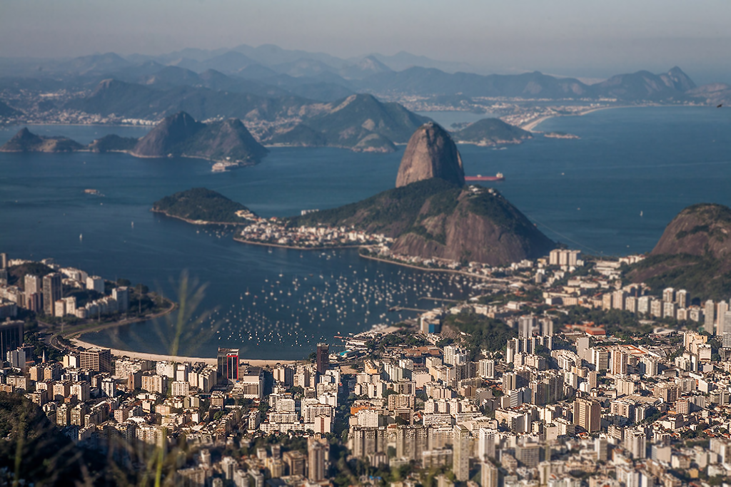
To create a nice tiltshift effect I looked for images of brazilian beaches on Creative Commons. I personally love the initiative, and if you want to learn a little more about how copyright works, I strongly recommend you to take a look at this fabolous post . During the serch, I found a lot of beautiful pictures of my country’s seashores. I needed to select one, but if you want to take a look at the pictures, I’ll leave a list of them at the end of this post

I will use “Brazil - A view of Rio de Janeiro from Christ the Redeemer” by sandeepachetan.com (licensed under CC BY-NC-ND 2.0). You can take a look at the image by clicking here. The image is saved in the project folder, and you can know more about my projects on OpenCV by following this link.

Let’s run the command line:

make ./exercises/tiltshift
./exercises/tiltshift exercises_images/Brazil_-_A_view_of_Rio_de_Janeiro_from_Christ_the_Redeemer.jpg

I played around with the sliders for a little bit. Here we have the result:

The first image is the ponder matrix and the second one is the complement of it. Notice that, in the areas one image is white, the other one is black, and vice-versa.

The last image is the result of the tiltshift effect. Notice how the most part of the image is blured, and only the area where the ponder matrix is white is on focus.

If you read until here, I would like to thank you for the patience and the curiosity. If you want to learn about what I am working with (AI or Computer Vision or whatever) please read another post (or don’t). :)

Images to Amaze yourself:

• Brazilian Beaches with Mountains

• Rio de Janeiro

• Biblioteca Real Gabinete Portugues de Leitura Rio de Janeiro Brazil

• Rio de Janeiro

• File:Vista aérea Centro do Rio de Janeiro RJ.jpg

• Brazilian Beach with Mountains