An ID3 implementation: Tree Class (Part 3/3)

In the previous two posts (Node Class and Math Functions) I explained the goal of the project and some concepts needed to make it work. Now it is time to finish this series introducing the Tree Class and how it will do the job of classifying instances.

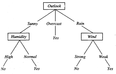
Decision Trees are created such that each internal node tests a feature and there are as many branches down this node as values in the feature tested. A classic example of Decision Tree represents the concept should I play Tennis today? making the following three questions: how is the outlook? (sunny, overcast or rain); how is the humidity? (high or normal) and how about the wind? (strong or weak).

Decision Tree for Should I Play Tennis?: Mitchell, p.53

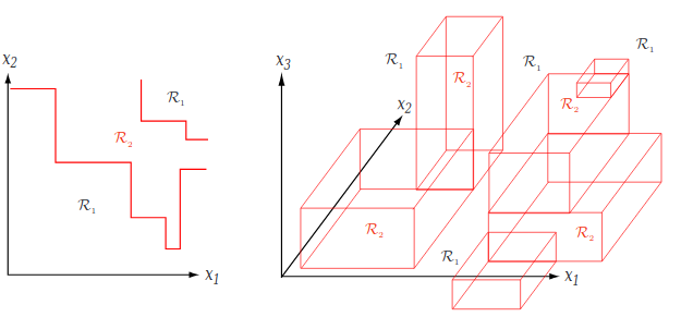
For numerical data, there is a simple way of visualizing how the decision tree makes decision: it creates hyperplane decision boundaries perpendicular to the coordinate axes.

Feature Space With Decision Boundaries: Duda, ch.8, p.8

It is important to mention there are more than just one algorithm for creating Decision Trees. As explained in the first post, I will focus on the Iterative Dichotommiser 3 algorithm (ID3).

The Algorithm

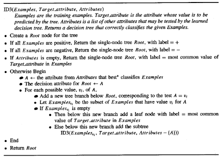
The Mini Project asks to generalize the ID3 algorithm (using split-stopping, though I did not implement it). Such classic algorithm can be seen below. It makes a tree that can classify instances in two disjoint classes.

ID3 Algorithm: Mitchell, p.56

A brief algorithm reading let us aware of some characteristics of Decision Tree Learning:

• Contructive and Eager Search: the tree is built by adding nodes, and this is all done in training time.
• Variable Size: any boolean function can be represented.

Now let’s understand a little about the parameters of the algorithm. It requires three specifications:

1. Examples: all the instances (features and labels)
2. Target_attribute: It indicates what value of the instance is the label. Imagine the Examples as a list where each row is an example. Target_attribute equalling last, for example, would indicate the last column is the label (attribute whose value is to be predicted by the tree).
3. Attributes: what attributes may be tested by the decision tree. During the Search for the best tree, the algorithm must be aware of what attributes are being used already, in order not to use any of them more than once. This parameter will do the job.

The algorithm is recursive. It returns nodes such that the last returned one will be the root, and all the others are internal nodes or leaf ones (created during recursion).

How does it work? The very first step is to create a node called root. Then the base cases are evaluated:

• All Examples are positive: then the current node must be a leaf with label +.
• All Examples are negative: then the current node must be a leaf with label -.
• All attributes were already tested: remember, each node tests a different feature. If they were all tested already, then the current node must be a leaf with a label that matches the most common value of the target attribute (label) in the dataset. This is done this way because the tree will be “guessing” with the most probable class to appear.

If the base cases are not matched, the algorithm enters the recursive case. Then, it must select the attribute that best classifies the Examples (remember Entropy from the second post?). It will be the attribute to be tested by the current node.

For each possible value of the chosen attribute there will be a branch down the node. The dataset (Examples) will be broken down such each of the the chunks will have a different possible value for the chosen attribute.

For each new branch the ID3 algorithm is called. It will receive the apropriate chunk of the dataset and a revised copy of the attributes to be tested (after removing the already tested attribute).

Code

Now let’s talk about how to implement the ID3 algorithm. The code will be written using Python and can be found here. The file has some imports and configurations at the beginning which can be ignored. That is why it will not be explained here.

For the sake of running the methods, it is important to use Numpy, the Node Class and the math functions file.

import numpy as np
from mtxslvnode import * 
from mtxslv_math_4_dt import *

The class has four methods and five attributes. A brief information about each of them can be found in the tables below (those marked with * are “private”).

Methods	Info
init	void constructor
fit	id3 algorithm initializer
mtxslv_id3*	id3 recursive algorithm implementation
evaluate	intance evaluation

Some methods worth of brief comments are fit, mtxslv_id3 and evaluate.

• fit: The method receives the features and labels, alongside with threshold. It calculates some values that need to be preset before id3. The threshold would be used with the pre-prunning, but this step was not implemented, so the value is not used anywhere.
• mtxslv_id3: the ID3 algorithm proper implementation. It also receives as parameters features, labels and threshold. It is a “private method” because I planned it not to be called outside the class inner working by any user.
• evaluate: it has the parameter instance (a collection of features). The parameter root has default value None, and is used in a recursive way (more details will be given down the post).

Attributes	Info
root	The Root Node for the Tree
node_quantity	How many nodes there exist
how_many_classes	How many classes there exist
number_of_classes	How many classes there exist
attributes_to_test*	What attributes can be tested

Here we go to some class attributes’ details.

• The difference between how_many_class and number_of_class lies in how they are used. The first one is used in the fit method, such t hat the information of how many classes exist can be retrieved later. The last one is used by the ID3 to know if any base case was met.
• The attributes_to_test is a boolean vector that indicates what attributes were already tested or not. Since each position in an instance is a feature (the vector is ordered), each position in the boolean vector relates to the respective instance attribute: if True, the instance attribute was not tested yet; if False, the instance attribute can be still tested. Notice it is the implementation of Attributes.
• node_quantity would be the amount of nodes there exist. I forget to implement it, unfortunately.

Now we can dive a little more in the class implementation.

class MtxslvDecisionTrees:
  def __init__(self):
    self.root = None
    self.node_quantity = 0
    self.how_many_classes = 0

  def fit(self, features, labels, threshold):
    self._attributes_to_test = [True for x in range(np.shape(features)[1])]
    self.number_of_classes = len(set(labels[:,0])) 
    self.root = self._mtxslv_id3(features,labels,threshold)

The constructor is void, and changes nothing about the class attributes.

The fit method updates the attributes_to_test class attribute as a boolean vector. It also counts how many classes there exist (notice this information is allocated in number_of_classes, not in how_many_classes). It updates the root node calling the mtxslv_id3 method.

def _mtxslv_id3(self, features, labels, threshold):
    current_node = MtxslvNode() 
    self.how_many_classes = len(set(labels[:,0])) 

    if((self.how_many_classes==1)):
      current_node.turn_node_to_leaf(-1,-1,most_common_class(labels))
      return current_node
    
    if(not(self._attributes_to_test.count(True))):  
      current_node.turn_node_to_leaf(-1,-1,most_common_class(labels))
      return current_node

    # watch out! There is no condition for empty feature set
    
    else:
      # this is the point in mitchell's id3 algorithm with "otherwise begin" 
      best_classifying_attribute = best_classifier_attribute(features,labels,self._attributes_to_test.copy()) 
      possible_attribute_values = set(features[:,best_classifying_attribute]) 
      self._attributes_to_test[best_classifying_attribute] = False
      for p_a_v in possible_attribute_values:
        features_vi, labels_vi = mtxslv_get_subset(features,labels,best_classifying_attribute,p_a_v)
        current_node.add_branch(best_classifying_attribute,p_a_v, self._mtxslv_id3(features_vi,labels_vi, threshold) )
    
    return current_node

I tried to imititate the ID3 algorithm while creating the mtxslv_id3. So the class method starts creating a node (MtxslvNode()). It also calculate how many classes exists (how many different values there exist in the label column?).

Now the code can go to the base conditions.

• There are only one class examples: this base condition is similar to “there are only positive or negative cases”. Since the class is a generalization for the binary algorithm, there is no need to think in terms of “only positive” or “only negative”. If there is only one class (self.how_many_classes==1), the current node is turned into a leaf and its label is the most common class labels has (do you remember the previous post?) . Then, the leaf is returned.
• There are no more attributes to be tested: each node must test a different attribute. If they were all tested already (then there are no True value in boolean vector self._attributes_to_test), the current node is turned into a leaf and has label the most common class the current dataset has.
• The dataset is empty: there is a base case where the dataset is empty. It was not implemented.

If no base case is met, the recursion case is then achieved. Let’s allocate and calculate the best_classifying_attribute and all the possible_attribute_values it can have (notice since the attribute will be used, it will no longer be “choseable”). Then, for each possible value in possible_attribute_values a branch will be added (each branch matches an attribute value). The branch will receive “as a node” the return of a mtxslv_id3 call. The new call has as dataset the chunk (method mtxslv_get_subset(), remember?) where the attribute to be tested has a particular value.

The last line of the method returns the current node. I don’t know if it will be executed (since the previous cases seem to account for all possibilities), but I wanted to implemented the ID3 algorithm completely.

The next method is the evaluation. It works recursevely: if the node is a leaf, return the label. If it is not, return a new call of the method, but with the next node that matches (the instance attribute has a particular value that leads down a particular branch, therefore a node).

def evaluate(self, instance, root = None):
  if (root == None):
    root = self.root
  if(root.is_leaf):
    return root.label
  else:
    attr_2_test = root.attribute_to_test
    instance_value = instance[attr_2_test]
    new_root = root.child_node[root.attribute_value.index(instance_value)]
    return self.evaluate(instance,new_root)

The default value of the parameter root is None and there is a conditional working on it in order to make the recursion work (class related issue). More explanations can be found here.

A Boolean Example

To illustrate the class, let’s suppose a concept (boolean function) defined as follows:

y = A and B or not(A)

The dataset related to this concept can be seen below.

A	B	y
0	0	1
0	1	1
1	0	0
1	1	1

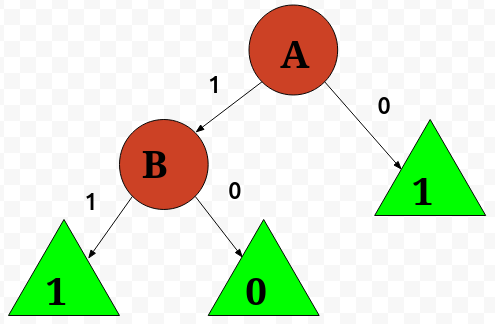
What I will do now on is to use the Decision Tree class I created to infer the concept of y Since Decision Trees can, at least, represent any boolean function, we can be sure the algorithm will find out rule that generated the dataset. Such resulting tree may look like the tree below. Let’s try to breafily read it. If A equals 0, then we go down to the leaf with label 1. Otherwise, if A equals 1, we need to assure B equals 1 as well, in order to go to label 1; else, we find ourselves with the label 0. Notice is just another way of reading the boolean concept defined above.

Boolean Decision Tree Example

Ok, let’s allocate the dataset and a tree object.

lista_features_coluna_1 = [[0],[0],[1],[1]]
lista_features_coluna_2 = [[0],[1],[0],[1]]
features_teste = np.concatenate((lista_features_coluna_1,lista_features_coluna_2), axis = 1)
labels_teste = np.array([[1],[1],[0],[1]])

arvore = MtxslvDecisionTrees()

Now let’s grow a tree out of the dataset. A threshold parameter must be given (though not used at all).

arvore.fit(features_teste, labels_teste, 0.05)

Now let’s see what I have got with these processings. First of all, what is stored in arvore.root?

arvore root

A MtxslvNode object, Great! Now I want to know if it is a leaf or not.

Is arvore root a leaf?

Not a leaf node. It should have some child nodes, then.

Are there child nodes?

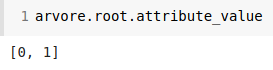
What attribute the root node tests?

What attribute to test?

It tests the attribute in the first column (remember, instances are zero based arrays). Such column is the attribute A, which can assume two values: zero and one.

What values the tested attribute can have?

Up to this momment we can be 100% sure the first node is right. Now we need to go down the tree to see if everything is fine.

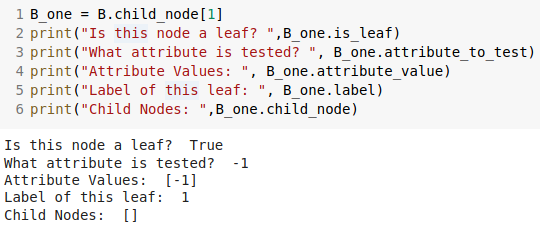
Let’s try to understand the node at the first list position.

Node at first list position characteristics.

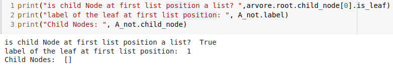
It is a leaf (with label 1), and is reached when the attribute A equals 0. Well, we are seeing the picture rightmost leaf!

What about the other root child node? It can only be the node that tests the attribute B!

Some queries to B node.

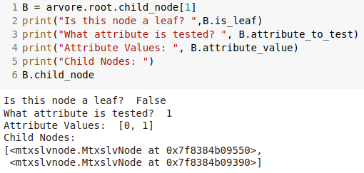
As can be seen, the attribute tested by the node is the second one (0 based list), which matches with that one I named B. It has two possible values, zero and one.

Ok, we can see the python class created a tree like that one in the picture so far. Let’s check the last two child nodes.

First Leaf down B node.

Second Leaf down B node.

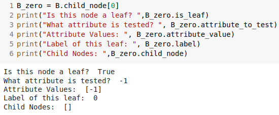
We see both these leaves has -1 value to the attribute to be tested and attribute value (actually, all leaves have this value, because of the implemented id3 algorithm).

The leaf reached when B equals 1 (and A equals 1) has label 1. The leaf reached when B equals 0 (and A equals 1) has label 0. They do not have child node as well, and it proves the class inner workings.

Final Discussion

Of course, the example above is a very special case (boolean concepts with well known dataset). But it proves the class works.

When I applied the algorithm to the project test dataset, I got ~27% of accuracy (that’s pretty low, sadly). The pre-prunning technique (chi-square test based) would be useful because it would bring this percentage up.

There’s a bug, also. If we try to evaluate the instance [4, 9, 6, 6, 3, 9, 8, 2, 8, 7, 6, 6, 0, 8, 4, 7], the console will throw an Exception that says the value 6 is not in a list.